How to evaluate the ‘goodness of fit’ of an EpiNow2 model run

forecasting

EpiNow2

Bayesian Analysis

Reproduction numbers

Stan

Published

November 8, 2025

library(EpiNow2)
library(posterior)
library(bayesplot)
library(data.table)
library(scoringutils)
library(dplyr)
library(ggplot2)

Introduction

This is a quick guide on how to assess or evaluate the output of an EpiNow2 model run.

EpiNow2 uses a Stan backend

{EpiNow2} uses Stan in the backend for model specification, fitting, and inference.

This means that the model fit can be assessed using the same tools and techniques used for any Stan model. The EpiNow2 package provides a convenient interface to run the models, but the underlying model is a Stan model.

The returned fit object is either a <stanfit> or CmdStanModel object, depending on the backend ({rstan} or {cmdstanr}) used. For example, you can use the {bayesplot} and {posterior} packages to visualize and summarize the model diagnostics.

Evaluating or assessing an {EpiNow2} model fit requires a holistic approach involving evaluating the MCMC diagnostics as well as the performance of the forecast against observed data. We will therefore proceed in that regard here.

Let’s start by setting up and running an example model, assessing the MCMC diagnostics, and then evaluating the forecast performance.

Running an example model

Input preparation

This will involve: loading required packages, setting up the model parameters, and running the model.

# Set number of cores for parallel processing.
options(mc.cores = min(4, parallel::detectCores() - 1))


# Set example generation time, incubation period, and reporting delay. In practice, these should use estimates from the literature or be estimated from data.
generation_time <- Gamma(
    shape = Normal(1.3, 0.3),
    rate = Normal(0.37, 0.09),
    max = 14
)

incubation_period <- LogNormal(
    meanlog = Normal(1.6, 0.06),
    sdlog = Normal(0.4, 0.07),
    max = 14
)
reporting_delay <- LogNormal(mean = 2, sd = 1, max = 10)

# Use example case data.

reported_cases <- example_confirmed[1:60]

# Plot the data
cases_plots <- ggplot(reported_cases, aes(x = date, y = confirm)) +
    geom_col() +
    labs(title = "Confirmed cases", x = "Date", y = "Cases") +
    theme_minimal()

cases_plots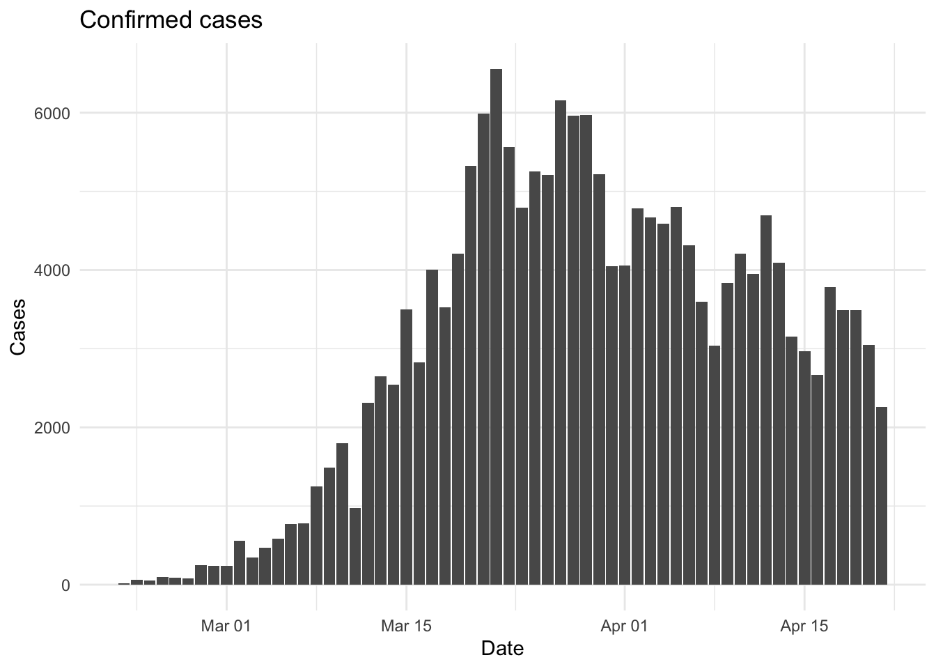

Fitting the model

Estimate Rt and nowcast/forecast cases by date of infection.

out <- epinow(
    data = reported_cases,
    generation_time = gt_opts(generation_time),
    rt = rt_opts(prior = LogNormal(mean = 2, sd = 0.1)),
    delays = delay_opts(incubation_period + reporting_delay)
)

Logging threshold set at INFO for the name logger
Writing EpiNow2 logs to the console and:
'/var/folders/vr/dn4r1_zj417drd1zr9301trw0000gp/T//RtmpMm2rHx/regional-epinow/2020-04-21.log'.
Logging threshold set at INFO for the name logger
Writing EpiNow2.epinow logs to the console and:
'/var/folders/vr/dn4r1_zj417drd1zr9301trw0000gp/T//RtmpMm2rHx/epinow/2020-04-21.log'.

# Plot the model fit
plot(out)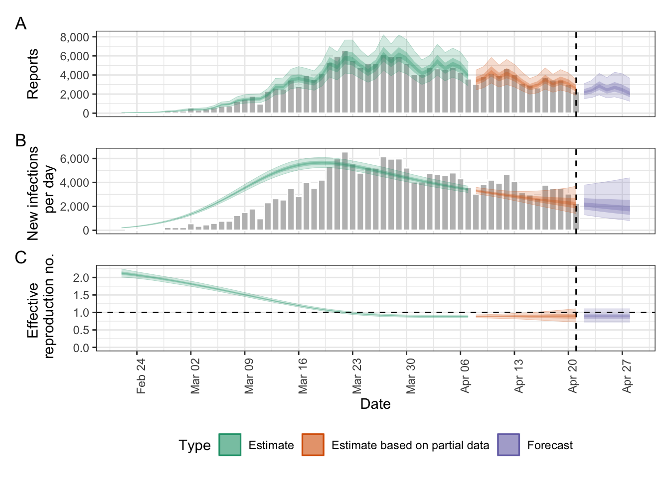

Assessing model diagnostics

We’ll first extract the Stan fit object and compute diagnostics. The epinow() function returns a list of model outputs, including the Stan fit object. This is what we need to assess the model fit. Stan provides diagnostic metrics to assess the model fit, convergence, etc. which we’ll use to assess the model fit. The Stan ecosystem has a rich set of tools for diagnosing model fit, including the bayesplot and posterior packages. These tools provide a way to visualize and summarize the model diagnostics. For an indepth look at MCMC diagnostics, for example, see the bayesplot R package vignette on visual MCMC diagnostics. You can also do posterior predictive checks using the bayesplot package.

Diagnostics include:

Divergent transitions. These should be minimized; ideally 0. Divergent transitions can be improved by tuning Stan controls like adapt_delta, max_treedepth, and stepsize in stan_opts(). If there are divergent transitions, increase adapt_delta (e.g., 0.95 or 0.99). See an in‑depth explanation at https://mc-stan.org/learn-stan/diagnostics-warnings.html.
Rhat. These should be close to 1 indicating good mixing. Rhat values should be less than 1.05 (See ?rstan::Rhat).
Treedepth. This should be low; high values indicate potential issues with the model.
ESS values. These should be high; low values indicate insufficient sampling. In particular, both bulk‑ESS and tail‑ESS should be at least ~100 per chain to ensure reliable posterior quantile estimates (see ?rstan::ess_bulk).

fit <- out$estimates$fit

np <- bayesplot::nuts_params(fit)
divergence_data <- subset(np, Parameter == "divergent__")
treedepth_data <- subset(np, Parameter == "treedepth__")

posterior_summary <- posterior::summarize_draws(
    fit, c(posterior::default_convergence_measures(), "ess_basic")
) |> subset(variable != "lp__")

fit_ess_basic <- min(posterior_summary$ess_basic, na.rm = TRUE)
fit_ess_bulk <- min(posterior_summary$ess_bulk, na.rm = TRUE)
fit_ess_tail <- min(posterior_summary$ess_tail, na.rm = TRUE)

diagnostics <- data.table(
    "samples" = nrow(np) / length(unique(np$Parameter)),
    "max_rhat" = round(max(posterior_summary$rhat, na.rm = TRUE), 3),
    "divergent_transitions" = sum(divergence_data$Value),
    "per_divergent_transitions" = mean(divergence_data$Value),
    "max_treedepth" = max(treedepth_data$Value),
    "ess_basic" = fit_ess_basic,
    "ess_bulk" = fit_ess_bulk,
    "ess_tail" = fit_ess_tail
)

diagnostics[, no_at_max_treedepth :=
                sum(treedepth_data$Value == max_treedepth)
][, per_at_max_treedepth := no_at_max_treedepth / samples]

knitr::kable(diagnostics)

samples	max_rhat	divergent_transitions	per_divergent_transitions	max_treedepth	ess_basic	ess_bulk	ess_tail	no_at_max_treedepth	per_at_max_treedepth
2000	1.01	0	0	9	1325.989	1277.945	1109.327	837	0.4185

Evaluating forecast performance

Forecast performance can be evaluated by comparing the forecast of reported cases with the observed cases using Proper Scoring Rules(Gneiting and Raftery 2007; Carvalho 2016) such as the Continuous Ranked Probability Score (CRPS) and Weighted Interval Score (WIS). These are available via the scoringutils::score() function.

The scoringutils::score() function requires a dataset that contains at least the following columns:

date: the date of the forecast
prediction: forecast values
true_value: the observed values
quantile: If evaluating quantiles, the quantile of the forecasted values (e.g., median, lower and upper bounds), in ascending order.

Let’s extract and prepare the forecasts and corresponding observed cases for the evaluation.

EpiNow2’s epinow() function returns a list of model outputs in the raw and several summarised formats for various use cases. In particular, there are time series of “infections”, “reported_cases”, “growth_rate”, and “R”, all grouped into “estimate”, “estimate based on partial data”, and “forecast”.

Here, we’re interested in the “forecast” type of the “reported_cases” variable, including the median and quantiles (lower and upper bounds).

# Extract the forecasts
forecasts <- out$estimates$summarised[variable == "reported_cases"][type == "forecast", ] %>% 
    select(-c(mean, sd, variable, strat, type))

Let’s also extract the corresponding subset of the observed data.

# Extract observed cases for the same period
obs_data <- example_confirmed[date >= min(forecasts$date) & date <= max(forecasts$date)]

Now, let’s combine the extracted forecasts with the observed data and clean up the quantiles into a format suitable for use with scoringutils. We will be cleaning them up because the forecasts data.table labels the quantiles as lower_20, upper_20, etc., where the number indicates the quantile level (e.g., 50% for the median), but that is not compatible with scoringutils.

# Combine forecasts with observed cases
eval_dt <- merge(forecasts, obs_data, by = "date")[, true_value := confirm][, confirm := NULL]

# Melt the data to long format
cols_to_melt <- c("median", grep("^(lower|upper)_", names(eval_dt), value = TRUE))
eval_long <- melt(
    eval_dt,
    id.vars = setdiff(names(eval_dt), cols_to_melt),
    measure.vars = cols_to_melt,
    variable.name = "prediction",
    value.name = "value"
)

# Prepare the evaluation data
eval_long[, quantile := fifelse(
  prediction == "median", 0.5,
  fifelse(
    grepl("^lower_", prediction),
    (1 - as.numeric(sub("lower_", "", prediction)) / 100) / 2,
    fifelse(
      grepl("^upper_", prediction),
      (1 + as.numeric(sub("upper_", "", prediction)) / 100) / 2,
      NA_real_
    )
  )
)][, prediction := value][, value := NULL]

Warning in fifelse(grepl("^lower_", prediction), (1 - as.numeric(sub("lower_",
: NAs introduced by coercion

Warning in fifelse(grepl("^upper_", prediction), (1 + as.numeric(sub("upper_",
: NAs introduced by coercion

# Sort the data by quantile
setorder(eval_long, quantile) %>% 
    head(10)

          date true_value prediction quantile
        <Date>      <num>      <num>    <num>
 1: 2020-04-22       2729    1526.00     0.05
 2: 2020-04-23       3370    1623.90     0.05
 3: 2020-04-24       2646    1911.95     0.05
 4: 2020-04-25       3021    1599.00     0.05
 5: 2020-04-26       2357    1701.95     0.05
 6: 2020-04-27       2324    1507.00     0.05
 7: 2020-04-28       1739    1237.85     0.05
 8: 2020-04-22       2729    1895.00     0.25
 9: 2020-04-23       3370    2056.75     0.25
10: 2020-04-24       2646    2420.00     0.25

Now we can use the scoringutils package to compute and summarise the scores. By default, a range of scores will be computed, including the interval_score, dispersion, underprediction, overprediction, coverage_deviation, bias, and ae_median.

# Mainly uses the scoringutils package
scored_scores <- eval_long[, quantile_level := quantile][, quantile := NULL][, model := "EpiNow2"] |> # align names to scoringutils preference
    as_forecast_quantile(observed  = "true_value", predicted = "prediction") |> 
    score() %>%
    summarise_scores()

Warning: ! Computation for `interval_coverage_90` failed. Error: ! To compute the
  interval coverage for an interval range of "90%", the 0.05 and 0.95 quantiles
  are required.

knitr::kable(scored_scores, digits = 3)

model	wis	overprediction	underprediction	dispersion	bias	interval_coverage_50	ae_median
EpiNow2	313.898	33.963	150.892	129.043	-0.143	0.571	444.286

Interpretation of scores

The table above provides a summary of the forecast performance by metrics. Note that it is not difficult to interpret the scores currently as they are not relative to other models. A proper comparison can only be done against other models.

Comparing against a baseline model

A common practice is to have a baseline model (Stapper and Funk 2025), such as a naive model, and compare the scores of your model against it.

Future updates

In future updates, I will explore more advanced techniques for model diagnostics and evaluation, including posterior predictive checks, cross-validation, and more using packages like loo, shinystan, and bayesplot

Resources

As this is a simple and basic guide, I’ll direct you to the following resources for more in-depth information on model diagnostics and forecast evaluation.

Stan’s guide on How to Diagnose and Resolve Convergence Problems
Understanding, evaluating, and improving forecasts of infectious disease burden open course.
scoringutils R package documentation
scoringRules R package documentation

References

Carvalho, Arthur. 2016. “An Overview of Applications of Proper Scoring Rules.” Decision Analysis 13 (4): 223–42.

Gneiting, Tilmann, and Adrian E Raftery. 2007. “Strictly Proper Scoring Rules, Prediction, and Estimation.” Journal of the American Statistical Association 102 (477): 359–78.

Stapper, Manuel, and Sebastian Funk. 2025. “Mind the Baseline: The Hidden Impact of Reference Model Selection on Forecast Assessment.” medRxiv, 2025–08.